Tags: Rotational Symmetry / Quadrupole Moment / Ellipsoidal coordinates
![]() The quadrupole moments of a homogeneously charged ellipsoid are calculated. The result will help us to understand how and why the quadrupole moments of an ellipsoidal charge distribution changes if it gets into an excited state.
The quadrupole moments of a homogeneously charged ellipsoid are calculated. The result will help us to understand how and why the quadrupole moments of an ellipsoidal charge distribution changes if it gets into an excited state.
Problem Statement
 Determine the quadrupole tensor
 for a homogeneously charged ellipsoid. The domain of the ellipsoid shall be mathematically given by
  i.e. its principal axes coincide with the coordinate axes.
- Assume the normalized charge distributions
 for "ground" and "excited" state, respectively. Here, s refers to the dimensionless radius variable in ellipsoidal coordinates (see hints).
Calculate the ratio of the nonvanishing quadrupole moments with respect to both states.
Hints
A suitable coordinate system are ellipsoidal coordinates given by
\[\begin{eqnarray*} x&=&as\sin\theta\cos\varphi\\y& = &bs\sin\theta\sin\varphi\\z&=&cs\cos\theta \end{eqnarray*}\ .\]
To perform the upcoming integrations, remember that the infinitesimal volume element changing coordinates transforms as
\[dxdydz = \det\left(\frac{\partial\left(x,y,z\right)}{\partial\left(s, \theta,\varphi\right)}\right)_{ij}dsd\theta d\varphi\].
It is not necessary to evaluate all quadrupole moments. Use that the quadrupole tensor is traceless and that we are already in a suitable coordinate system.
You may find the formula \(\int_{0}^{\infty}s^{n} e^{-s/s_{0}}ds = n!\,s_{0}^{n+1}\) for \(s_0 >0\) quite useful at some point.
Solution ✔
The calculation of multipole moments from sources generally involves integration techniques. Using the appropriate ellipsoidal coordinates we will find the quadrupole moments of the ellipsoid fastly. Afterwards, we can use our findings to quickly compare the hypothized charge distributions. If you want to find out more about how quadrupole moment investigations lead to a better understanding of atomic nuclei, please have a look at "A Simple Model for Atomic Nuclei: The Deformed Sphere and its Multipole Moments".
Calculation of the Quadrupole Moments - Homogeneous Ellipsoid
The integral equation we have to solve to find the quadrupole moments is given by
\[Q_{ij}= \int\left(3x_{i}^{\prime} x_{j}^{\prime}-r^{\prime2}\delta_{ij}\right) \rho\left(\mathbf{r}^{\prime}\right)d^{3} \mathbf{r}^{\prime}\ .\]
To simplify the integration over the ellipsoid to a great extent, we use ellipsoidal coordinates. In this coordinate system, the infinitesimal volume element can be calculated as
\[\begin{eqnarray*} dxdydz&=&\det\left(\frac{\partial\left(x,y,z\right)}{\partial \left(s,\theta,\varphi\right)}\right)_{ij}dsd \theta d\varphi\\& = &\det\left(\begin{array}{ccc}a\sin\theta\cos\varphi & as\cos\theta\cos\varphi & -as\sin\theta\sin\varphi\\b \sin\theta\sin\varphi & bs\cos\theta\sin\varphi & bs\sin\theta\cos\varphi\\c\cos\theta & -cs\sin\theta & 0\end{array}\right)dsd\theta d \varphi\\& = &abcs^{2}\sin\theta dsd\theta d\varphi \end{eqnarray*}\ .\]
after some steps of matrix reduction. Naturally, we would have directly expected such a result with respect to the volume element in spherical coordinates.
Let us consider the diagonal multipole moments first. Since the quadrupole tensor is traceless, i.e. \(\sum_{i}Q_{ii}=0\), we just have to calculate the xx and yy moments directly to find the zz moment. Following the definition of the quadrupole moments, we have to calculate
\[\begin{eqnarray*} Q_{xx}&=&\rho_{0}\int_{\Omega}\left[3x^{\prime2}- \left(x^{\prime2}+y^{\prime2}+z^{\prime2}\right) \right]dx^{\prime}dy^{\prime}dz^{\prime}\\& = &\rho_{0}abc\int_{\Omega}\left(2a^{2}\sin^{2}\theta\cos^{2}\varphi-b^{2}\sin^{2}\theta\sin^{2}\varphi-c^{2}\cos^{2}\varphi\right)s^{{\color{red}4}}\sin\theta dsd\theta d\varphi\ . \end{eqnarray*}\]
The integration for \(s\) from zero to one is simple and yields \(1/5\), \(\int_{0}^{1}s^{4}ds=1/5\), and we may proceed with the angular terms. Nevertheless, let us write down some basic integration results that will help us to find all results fastly:
\[\begin{eqnarray*} \int_{0}^{2\pi}\sin^{2}\varphi d\varphi&=&\left[\frac{1}{2}\varphi-\frac{1}{4}\sin2\varphi\right]_{0}^{2\pi}=\pi\ ,\\\int_{0}^{2\pi}\cos^{2}\varphi d\varphi& = &\left[\frac{1}{2}\varphi+\frac{1}{4}\sin2\varphi\right]_{0}^{2\pi}=\pi\ ,\\\int_{0}^{\pi}\sin^{3}\theta d\theta & = & \left[-\cos\theta+\frac{1}{3}\cos^{3}\theta\right]_{0}^{\pi} = \frac{4}{3}\ \mathrm{and}\\\int_{0}^{\pi}\sin \theta\cos^{2}\theta d\theta& = &\left[-\frac{1}{3}\cos^{3}\theta\right]_{0}^{\pi}=\frac{2}{3}\ . \end{eqnarray*}\]
We find, first integrating over \(\theta\) and then \(\varphi\):
\[\begin{eqnarray*} Q_{xx}&=&\frac{1}{5}\rho_{0}abc\int_{0}^{2\pi}\int_{0}^{\pi}\left(2a^{2}\underbrace{\sin^{2}\theta}_{4/3}\cos^{2}\varphi-b^{2}\underbrace{\sin^{2}\theta}_{4/3}\sin^{2}\varphi-c^{2} \underbrace{\cos^{2}\varphi}_{2/3}\right){\color{red}\sin\theta}d\theta d\varphi\\& = &\frac{1}{15}\rho_{0}abc\int_{0}^{2\pi}\left(8a^{2}\underbrace{\cos^{2} \varphi}_{\pi}-4b^{2}\underbrace{\sin^{2} \varphi}_{\pi}-2c^{2}\right)d \varphi\\& = &\frac{4\pi}{15}\rho_{0}abc\left[2a^{2}-b^{2}-c^{2}\right]\ . \end{eqnarray*}\]
The calculation of \(Q_{yy}\) follows analogously:
\[\begin{eqnarray*} Q_{yy}&=&\frac{1}{5}\rho_{0}abc\int_{0}^{2\pi}\int_{0}^{\pi}\left(2b^{2} \underbrace{\sin^{2}\theta}_{4/3}\underbrace{\sin^{2}\varphi}_{\pi}-a^{2} \underbrace{\sin^{2}\theta}_{4/3}\underbrace{\cos^{2}\varphi}_{\pi}-c^{2}\underbrace{\cos^{2}\varphi}_{2/3}\right) \sin\theta d\theta d\varphi\\& = &\frac{4\pi}{15}\rho_{0}abc\left(2b^{2}-a^{2}-c^{2}\right)\ . \end{eqnarray*}\]
As proclaimed, we may now simply use the vanishing trace of the quadrupole tensor to find
\[Q_{zz} = \frac{4\pi}{15}\rho_{0} abc\left(2c^{2}-a^{2}-b^{2}\right)\ .\]
The off-diagonal moments should all vanish since we are already in a coordinate system where the axes of the ellipsoid are coinciding with the coordinate axes. Let us see if this is true at the example of the xy moment:
\[\begin{eqnarray*} Q_{xy}&=&3\int x^{\prime}y^{\prime}\rho\left(\mathbf{r}^{\prime}\right)d^{3} \mathbf{r}^{\prime}\\& = &3\rho_{0}ab\int_{\Omega}\sin\theta\cos\varphi\, \sin\theta\sin\varphi\, s^{4}\sin\theta dsd\theta d\varphi\\&=&\frac{3}{5}\rho_{0}ab\int \int\sin^{3}\theta\underbrace{\cos\varphi\sin\varphi}_{1/2\sin2\varphi}d\theta d\varphi\\& = &0\ \surd \end{eqnarray*}\]
Finally we can conclude that the quadrupole tensor of an ellipsoid with a homogeneous mass distribution is given by
\[\begin{eqnarray*} Q&=&\frac{q}{5}\left(\begin{array}{ccc}2a^{2}-b^{2}-c^{2} & 0 & 0\\0 & 2b^{2}-a^{2}-c^{2} & 0\\0 & 0 & 2c^{2}-a^{2}-b^{2}\end{array}\right)\ \mathrm{with}\\q&=&\frac{4\pi}{3}abc\,\rho_{0}\ , \end{eqnarray*}\]
the total charge of the ellipsoid.
Quadrupole Moments: Excited vs. Ground State
The first integration we performed to find the quadrupole tensor of a homogeneously charged ellipsoid was an integration over the dimensionless radial coordinate \(s\). Furthermore, because of the suited coordinate system, any other integration was totally independent. This leads to the following situation if we change the charge distribution only with respect to \(s\): we have to replace
\[\frac{1}{5}\rho_{0} \rightarrow \int_{0}^{\infty}\rho\left(s\right)s^{4}ds\ ,\]
since no other integration is affected at all!
Thus, in the case of the "ground state", we calculate
\[\begin{eqnarray*} \frac{1}{5}\rho_{0}& \rightarrow&\int_{0}^{\infty}\rho\left(s\right)s^{4}ds\\& = &\tilde{\rho}_{0}\frac{4}{s_{0}^{3}}\int_{0}^{\infty}e^{-2s/s_{0}}s^{4}ds \\ &=& \tilde{\rho}_{0}\frac{4}{s_{0}^{3}}4!\left(\frac{s_{0}}{2}\right)^{5}= 3\, s_{0}^{2}\tilde{\rho}_{0} \end{eqnarray*}\]
and in the case of the "excited state" the integration changes via
\[\begin{eqnarray*} \frac{1}{5}\rho_{0}&\rightarrow& \int_{0}^{\infty}\rho\left(s\right)s^{4}ds\\& = &\int_{0}^{\infty}\tilde{\rho}_{0}\frac{1}{3}\frac{1}{\left(2s_{0}\right)^{3}}\left(\frac{s}{s_{0}}\right)^{2}e^{-s/s_{0}}s^{4}ds\\& = &\frac{1}{24s_{0}^{5}}\tilde{\rho}_{0}\int_{0}^{\infty}e^{-s/s_{0}}s^{6}ds\\& = &\frac{6!s_{0}^{7}}{24s_{0}^{5}}\tilde{\rho}_{0} = 30\, s_{0}^{2}\tilde{\rho}_{0}\ . \end{eqnarray*}\]
We find that via excitation the quadrupole moment of the ellipsoidal charge distribution is enhanced by a factor of ten. This is a behaviour we somehow expected: the charge density of the excited state is more distant to the center than for the ground state, see figure below. By definition of the quadrupole tensor with moments \(\propto x_{i}^{\prime}x_{j}^{\prime}\rho\left(\mathbf{r}^{\prime}\right)\), such a higher displacement of the charge density causes a higher quadrupole moment.
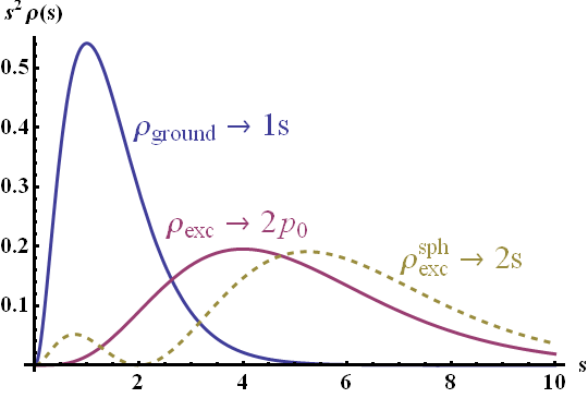
Illustration of the used ground and excited state charge densities \(\rho_i\left(s\right)\). The ground state (blue line) has a much higher probability close to the center than the excited state (magenta line).
Please note that a more correct analogon for the excited and ground state would be to use the radial dependency
\[\rho_{\mathrm{exc}}^{\mathrm{sph}}\left(s\right) = \tilde{\rho}_{0}\frac{1}{8 s_{0}^{3}} e^{-s/s_{0}}\left(2-s/s_{0}\right)^2 ,\]
which is related to the spherically symmetric 2s state of the Hydrogen atom (with \(r \rightarrow s\)) and leads to a 14-fold enhancement. The employed form of the excited state corresponds to a 2p0 state of the Hydrogen atom and obeys a slightly more complicated angular dependency. Here it was chosen for simplicity.


