The Magnetic Field of an Infinite Wire

One of the basic problems of magnetostatics is the infinite wire. Using the several symmetries of the current distribution we will be able to not only find the magnetic field - we will also verify the "right-hand rule".

Problem Statement

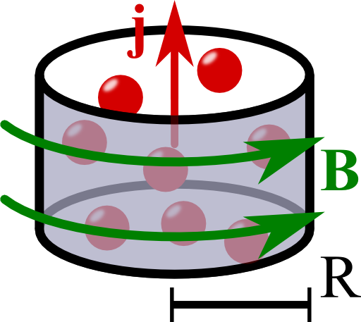Calculate the magnetic field of an infinitely long wire with a uniform current distribution

in the following way:

1. Explain why the magnetic field for the given current distribution only depends on ρ (cylindrical coordinates), i.e. why B(r) = B(ρ).
2. Additional - Verify the “right-hand-rule”: - if a current distribution is generally given by j(ρ)e_z (translation and rotation symmetry), show that the magnetic field can only have an angular component φ.
3. Use the integral form of Ampère's law to calculate the magnetic field everywhere.

Note that we use mostly differential methods to calculate the fields everywhere in this problem. In "The Magnetic Field due to a Thin Infinite Wire" we use the Biot-Savart law (integration!) to determine the magnetic field.

Nevertheless, our general solution here is also valid with respect to thin wires if we let R → 0.

Hints

The curl of a vector field in cylindrical coordinates is given by

You cannot use the thin-wire Biot-Savart here. Maybe you find use for Stoke's theorem,

Solution ✔

Let us determine the magnetic field for uniform current in the wire using all of the symmetries that are given in the system. First of all, let us find that \(\mathbf{B}\) can only depend on the (cylindrical) radial coordinate. With this result, we will easily be able to verify the right-hand rule for a general class of current distributions. The solution will then be a last easy step using Stoke's theorem.

Translation and Rotation Symmetries: \(\mathbf{B}\left(\mathbf{r}\right)=\mathbf{B}\left(\rho\right)\)

Ampere's law relates the magnetic induction \(\mathbf{B}\left(\mathbf{r}\right)\) and the current density \(\mathbf{j}\left(\mathbf{r}\right)\): \[\nabla\times\mathbf{B}\left(\mathbf{r}\right) = \mu_{0}\mathbf{j}\left(\mathbf{r}\right)\ .\]Note that for non-magnetic media, the magnetic field \(\mathbf{H}\) is related to the magnetic induction by \(\mathbf{B}\left(\mathbf{r}\right)=\mu_{0}\mathbf{H}\left(\mathbf{r}\right)\). Then, we may also call \(\mathbf{B}\) magnetic field. The given current distribution (in cylindrical coordinates),\[\mathbf{j}\left(\mathbf{r}\right) = \begin{cases}j_{0} & \rho\leq R\\0 & \mathrm{else}\end{cases}\mathbf{e}_{z}\ ,\]obeys a translational symmetry - there is no change of the current along the z coordinate.

This means, that the magnetic field cannot depend on this coordinate - the current is its source! Furthermore, we find that \(\mathbf{j}\) is rotationally symmetric - there is no explicit dependence on the angular coordinate \(\varphi\) (remember that i.e. \(x=\rho\cos\varphi\)). Hence, also the magnetic field cannot depend on \(\varphi\)! So we know that the magnetic field has to be given by\[\mathbf{B}\left(\mathbf{r}\right) \equiv \mathbf{B}\left( \rho \right)\ .\]We may now go a little further exploiting the symmetries to verify the “right-hand rule”.

Verification of the Right-Hand Rule

Let us convince ourselves that the magnetic field can only have an angular component if\[\mathbf{j}\left(\mathbf{r}\right) = j\left(\rho\right)\mathbf{e}_{z}\ .\]We need to consider the curl of \(\mathbf{B}\) in Ampère's law directly. In suitable cylindrical coordinates we find\[\begin{eqnarray*} \nabla\times\mathbf{B}\left(\rho\right)&=&\left(\frac{1}{\rho}{\color{red}{\partial_{\varphi}B_{z}\left(\rho\right)}}-\color{red}{\partial_{z}B_{\varphi}\left(\rho\right)}\right)\mathbf{e}_{\rho}+\left({\color{red}{\partial_{z}B_{\rho}\left(\rho\right)}}-\partial_{\rho}B_{z}\left(\rho\right)\right)\mathbf{e}_{\varphi}\\&&+\frac{1}{\rho}\left(\partial_{\rho}\left[\rho B_{\varphi}\left(\rho\right)\right]-{\color{red}{\partial_{\varphi}B_{\rho}\left(\rho\right)}}\right)\mathbf{e}_{z}\\&=&-\partial_{\rho}B_{z}\left(\rho\right)\mathbf{e}_{\varphi}+\frac{1}{\rho}\partial_{\rho}\left[\rho B_{\varphi}\left(\rho\right)\right]\mathbf{e}_{z}\ . \end{eqnarray*}\]Here we have highlighted terms in red that vanish since \(\mathbf{B}\left(\mathbf{r}\right)=\mathbf{B}\left(\rho\right)\) also holds for the slightly more general current distribution (same symmetries!).

Furthermore, our current density has only a component in z direction. By Ampère's law, the same has to hold for the curl of the magnetic field! From the latter equation, we see that the \(\mathbf{e}_{\varphi}\) component of the curl of the magnetic field has to vanish. Hence, \(\partial_{\rho}B_{z}\left(\rho\right)=0\). Also, since the magnetic field should vanish for \(\rho\rightarrow\infty\), \[B_{z}\left(\rho\right) \equiv 0\ .\]Now we can be convinced that the magnetic field can only have an angular component \(B_{\varphi}\left(\rho\right)\) for charge distributions with translational and rotational symmetry! In general, symmetries are very powerful and can be used to simplify problems to a great extend, see also "A Cylinder Shell Current and its Magnetic Field".

So, we have really verified the right-hand rule: a current represented by the thumb results in a magnetic field following the fingers of our right hand.

It's time to determine the magnetic field!

Calculation of the Magnetic Field

If we integrate Ampère's law over a two-dimensional surface \(\Omega\), we can apply Stoke's theorem to find the integral version of Ampère's law:\[\begin{eqnarray*} \int_{\Omega}\nabla\times\mathbf{B}\left(\mathbf{r}\right)d\mathbf{A}&=&\int_{\Omega}\mu_{0}\mathbf{j}\left(\mathbf{r}\right)d\mathbf{A}\ ,\ \text{so}\\\oint_{\partial\Omega}\mathbf{B}\left(\mathbf{r}\right)d\mathbf{r}&=&\int_{\Omega}\mu_{0}\mathbf{j}\left(\mathbf{r}\right)d\mathbf{A}\ . \end{eqnarray*}\]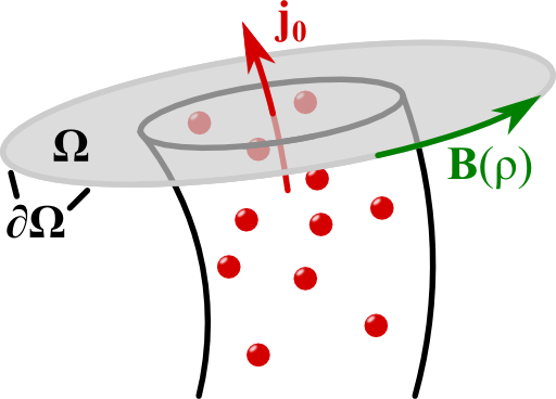

Of course we are clever and take a circular surface. Here, the boundary is given by some fixed radius \(\rho\) where the magnetic field is constant. Then,\[\begin{eqnarray*}\oint_{\partial\Omega}\mathbf{B}\left(\mathbf{r}\right)d\mathbf{r}&=&\oint_{\partial\Omega}B_{\varphi}\left(\rho\right)\rho d\varphi=2\pi\rho B_{\varphi}\left(\rho\right)\ \text{and}\\\int_{\Omega}\mu_{0}\mathbf{j}\left(\mathbf{r}\right)d\mathbf{A}&=&\mu_{0}\begin{cases}\pi\rho^{2}j_{0} & \rho\leq R\\\pi R^{2}j_{0} & \text{else}\end{cases}\ .\end{eqnarray*}\]The result for the integration over the whole wire is also the total electric current\[I = \int_{\text{wire}}\mu_{0}\mathbf{j}\left(\mathbf{r}\right)d\mathbf{A}=\pi R^{2}j_{0}\ .\]We conclude that the magnetic field is finally given as\[\begin{eqnarray*} \mathbf{B}\left(\mathbf{r}\right)&=&\mathbf{e}_{\varphi}\frac{\mu_{0}}{2\pi\rho}\begin{cases}\pi\rho^{2}j_{0} & \rho\leq R\\\pi R^{2}j_{0} & \rho>R\end{cases}\\&=&\mathbf{e}_{\varphi}\frac{\mu_{0}I}{2\pi\rho}\begin{cases}\frac{\rho^{2}}{R^{2}} & \rho\leq R\\1 & \text{else}\end{cases}\ . \end{eqnarray*}\]Note that the result of an infinitely thin wire is also reproduced for \(\rho\geq R\).

We can also see what we had to do if the current distribution was a more complicated function of \(\rho\). We would have to simply integrate inside the wire to find the magnetic field there. Outside of the wire it becomes evident that the only important parameter is indeed the current - the field will always look like if it was originated from an infinitely thin wire. Of course this sounds familiar if we remember "The Electric Field of a Point Charge", where the field outside of a radially symmetric charge distribution is entirely determined by the net charge.