Tags: Far Field / Radiation pattern
![]() Antenna arrays are an important class of antennas which are widely used in point to point communication systems, where a very high directive beam of radiation is needed. In The Finite Dipole Antenna we saw that a dipole antenna has an omnidirectional pattern which has a very low directivity. In this problem we will see how to arrange several dipole antennas into an array to obtain a directive radiation pattern.
Antenna arrays are an important class of antennas which are widely used in point to point communication systems, where a very high directive beam of radiation is needed. In The Finite Dipole Antenna we saw that a dipole antenna has an omnidirectional pattern which has a very low directivity. In this problem we will see how to arrange several dipole antennas into an array to obtain a directive radiation pattern.
Problem Statement
Assume an array of antennas which consists of \(N\) half-wavelength dipoles working at \(300\, \mathrm{MHz}\). The dipoles are located with exactly the same orientation at positions which are given by
\[\mathbf{r}_n=n\, d\,\mathbf{e}_z\,, \quad n=\{0,1,2,...,N-1\} \]
where \(d\) is the distance between two adjacent dipoles. In addition, each dipole has a feed current which is given by
\[\tilde{I}_n=I_n e^{-\mathrm{i}n\phi_0}\,, \quad n=\{0,1,2,...,N-1\}\]
where \(\phi_0\) is a fixed parameter which is called the progressive phase.
- Find the array factor for an array with 6 elements (N=6) with spacing of \(\lambda/2\) (\(d=\lambda/2\)).
The elements have uniform amplitude with progressive phase of zero (i.e. \(\tilde{I}_n=I_0\)). - Sketch the array pattern in y-z plane.
- Calculate the first-null beamwidth (FNBW) and side lobe level (SLL) of the array pattern.
- Sketch the overall pattern of the array while all dipoles are oriented in x-direction.
Hints: Far Field and Array Pattern
- Find far fields using the following formulas:
Vector potential:
\[\begin{equation*} \mathbf{A}(\mathbf{r},\omega)=\frac{\mu\,e^{\mathrm{i} k r}}{4\pi r}\int_{V'}\mathbf{j}\left(\mathbf{r'},\omega\right) e^{-\mathrm{i} k\, \mathbf{r'}.\,\mathbf{e}_r}dV'\ \end{equation*}\]Magnetic field:
\[\begin{equation*} \mathbf{H}\left(\mathbf{r},\omega\right)=\frac{1}{\mu}\mathrm{i}k\mathbf{e}_r\times\mathbf{A}\left(\mathbf{r},\omega\right)\ \end{equation*}\]Electric field:
\[\begin{equation*} \mathbf{E}\left(\mathbf{r},\omega\right)=\mathrm{i}\omega\mathbf{A^t}\left(\mathbf{r},\omega\right) \end{equation*}\]
where \(\mathbf{A^t}\left(\mathbf{r},\omega\right)\) is the tangential component of \(\mathbf{A}\left(\mathbf{r},\omega\right)\).
Then, try to decompose far fields into two parts: 1) element contribution (element factor) and 2) array contribution (array factor) - Note that the array pattern is rotationally symmetric.
- First-null beamwidth is defined as the angular distance between the adjacent nulls to the main lobe, and side lobe level is the ratio of the amplitude of the second largest lobe to the amplitude of the main lobe.
- The overall pattern of the array can be obtained by multiplying the element pattern (dipole pattern) and array pattern.
Solution: Array Pattern of Phased Antenna Array
Consider a general antenna array which consist of N elements. Each element has the following current distribution
\[\mathbf{j}_n\left(\mathbf{r},\omega\right)=I_n e^{-\mathrm{i}\phi_n}\mathbf{j}\left(\mathbf{r}-\mathbf{r_n},\omega\right)\,, \quad n=\{0,1,2,...,N-1\}\] where \(\mathbf{r_n}\) is the location of the \(\mathrm{n^{th}}\) element. This means that all elements have the same current distribution (\(\mathbf{j}\left(\mathbf{r},\omega\right)\)) but their phases, amplitudes, and locations are different.
Therefore, the current distribution for the array can be written as shown below.
\[\begin{equation} \mathbf{j}_t\left(\mathbf{r},\omega\right)=\sum_{n=0}^{N-1} I_n e^{-\mathrm{i}\phi_n}\mathbf{j}\left(\mathbf{r}-\mathbf{r_n},\omega\right) \end{equation}\]
Using this current distribution one can easily calculate the vector potential as follows. \begin{eqnarray} \mathbf{A}(\mathbf{r},\omega)&=&\frac{\mu\,e^{\mathrm{i} k r}}{4\pi r}\int_{V'}\mathbf{j}_t\left(\mathbf{r'},\omega\right) e^{-\mathrm{i} k\, \mathbf{r'}.\,\mathbf{e}_r}dV'\nonumber\\&=&\frac{\mu\,e^{\mathrm{i} k r}}{4\pi r} \sum_{n=0}^{N-1} I_n e^{-\mathrm{i}\phi_n}\int_{V'}\mathbf{j}\left(\mathbf{r'}-\mathbf{r_n},\omega\right) e^{-\mathrm{i} k\, \mathbf{r'}.\,\mathbf{e}_r}dV'\nonumber \end{eqnarray} which can be simplified using change of variables (\(\mathbf{r'}-\mathbf{r_n}=\mathbf{r''}\)) as follows. This equation shall be labeled "AR".
\[\begin{eqnarray} \mathbf{A}(\mathbf{r},\omega)&=&\frac{\mu\,e^{\mathrm{i} k r}}{4\pi r} \sum_{n=0}^{N-1} I_n e^{-\mathrm{i}\phi_n}\int_{V''}\mathbf{j}\left(\mathbf{r''},\omega\right) e^{-\mathrm{i} k\,\left(\mathbf{r''}+\mathbf{r_n}\right)\cdot\,\mathbf{e}_r}dV''\nonumber\\&=&\left[\frac{\mu\,e^{\mathrm{i} k r}}{4\pi r} \int_{V''}\mathbf{j}\left(\mathbf{r''},\omega\right) e^{-\mathrm{i} k\,\mathbf{r''}\cdot\,\mathbf{e}_r}\,dV''\right]\,\left[\sum_{n=0}^{N-1} I_n e^{-\mathrm{i}\phi_n}e^{-\mathrm{i} k\,\mathbf{r_n}\cdot\,\mathbf{e}_r}\right]\nonumber\\&=&\mathbf{A}_e(\mathbf{r},\omega)\,R(\theta,\phi) \end{eqnarray}\]
where:
\[\begin{eqnarray} &&\mathbf{A}_e(\mathbf{r},\omega)=\frac{\mu\,e^{\mathrm{i} k r}}{4\pi r} \int_{V''}\mathbf{j}\left(\mathbf{r''},\omega\right) e^{-\mathrm{i} k\,\mathbf{r''}\cdot\,\mathbf{e}_r}\,dV''\nonumber\\&& R(\theta,\phi)=\sum_{n=0}^{N-1} I_n e^{-\mathrm{i}\phi_n}e^{-\mathrm{i} k\,\mathbf{r_n}\cdot\,\mathbf{e}_r} \end{eqnarray}\]
We shall call the former equation "R". As can be seen, \(\mathbf{A}_e(\mathbf{r},\omega)\) is just the vector potential of a single element in array which is located at the center of the coordinate system.
Therefore, the vector potential of the array in nothing but the vector potential of a single element of the array multiplied by a function (\(R(\theta,\phi)\)) which we call it array factor. It is apparent that the array factor depends only on the geometry of the array and the relative phase and amplitude of the elements, but not the shape and properties of the elements (the elements can be horn antennas, dipoles, helix antennas, etc, with exactly the same array factor).
Using Eq. [AR], the far fields can be obtained easily. Equations "HR" and "ER" are given as:
\[\begin{eqnarray} \mathbf{H}\left(\mathbf{r},\omega\right)&=&\frac{1}{\mu}\mathrm{i}k\mathbf{e}_r\times\mathbf{A}\left(\mathbf{r},\omega\right)\nonumber\\&=&\frac{1}{\mu}\mathrm{i}k\mathbf{e}_r\times\left[\mathbf{A}_e(\mathbf{r},\omega)\,R(\theta,\phi)\right]\nonumber\\&=&\mathbf{H}_e(\mathbf{r},\omega)\,R(\theta,\phi)\end{eqnarray}\]
\[\begin{eqnarray} \mathbf{E}\left(\mathbf{r},\omega\right)&=&\mathrm{i}\omega\mathbf{A^t}\left(\mathbf{r},\omega\right)\nonumber\\&=&\mathrm{i}\omega\left[\mathbf{A}_e^t(\mathbf{r},\omega)\,R(\theta,\phi)\right]\nonumber\\&=&\mathbf{E}_e(\mathbf{r},\omega)\,R(\theta,\phi) \end{eqnarray}\]
where, \(\mathbf{E}_e\) and \(\mathbf{H}_e\) are far fields of a single element.
Furthermore, Poynting vector can also be calculated using Eq. [HR] and [ER]. This gives us equation "SR":
\[\begin{eqnarray} \mathbf{S}\left(\mathbf{r},\omega\right)&=&\frac{1}{2}\,\Re\Big\{\mathbf{E}\left(\mathbf{r},\omega\right)\times \mathbf{H^*}\left(\mathbf{r},\omega\right)\Big\} \nonumber\\&=&\frac{1}{2}\,\Re\Big\{\mathbf{E}_e\left(\mathbf{r},\omega\right)\times \mathbf{H}_e^*\left(\mathbf{r},\omega\right)\Big\}\,|R(\theta,\phi)|^2 \nonumber\\&=&\mathbf{S}_e\left(\mathbf{r},\omega\right)\,|R(\theta,\phi)|^2 \end{eqnarray}\]
As can be seen in Eq. [SR], the antenna pattern (radial component of the Poynting vector) is the multiplication of the element pattern and the array pattern. Note that the array pattern is independent of the element pattern. Therefore, it can be designed and analyzed, regardless of the type of the elements.
Now let us calculate the array factor for the array given in this problem. Using Eq. [R] we obtain
\[\begin{eqnarray} R(\theta,\phi)&=&\sum_{n=0}^{5} I_n e^{-\mathrm{i}\phi_n}e^{-\mathrm{i} k\,\mathbf{r_n}\cdot\,\mathbf{e}_r}\nonumber\\&=&I_0\sum_{n=0}^{5} e^{-\mathrm{i} k\,n\, d\,\mathbf{e}_z\cdot\,\mathbf{e}_r}=I_0\sum_{n=0}^{5} e^{-\mathrm{i} k\,n\,\frac{\lambda}{2}\,\cos(\theta)}\nonumber\\&=&I_0\,\frac{1-e^{-\mathrm{i}\, 6\pi\,\cos(\theta)}}{1-e^{-\mathrm{i}\, \pi\,\cos(\theta)}}\nonumber \end{eqnarray}\]
\[\begin{equation} \Rightarrow\mathrm{Array Pattern:}\quad |R(\theta,\phi)|^2=I_0^2 |\frac{\sin\left(\frac{6}{2}\pi\,\cos(\theta)\right)}{\sin\left(\frac{1}{2}\pi\,\cos(\theta)\right)}|^2 \end{equation}\]
The latter equation shall be termed "AP1". The array factor is plotted in Fig. [1] (note that the figure is plotted in dB in order to make the small side lobes visible).
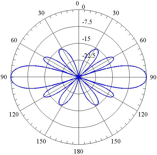
As can be seen the pattern has four side lobes and six nulls. Using Eq. [AP1], the nulls can be calculated easily. \[|R(\theta,\phi)|^2=0\quad\rightarrow \quad Nulls:\quad \theta_\text{n}\simeq\{0,48.2^\circ,70.5^\circ,109.5^\circ,131.8^\circ,180^\circ\}\] Therefore, \[\mathrm{FNBW}=109.5^\circ-70.5^\circ=39^\circ\] which is approximately one fifth of the FNBW of a half-wavelength dipole.
To calculate the SLL, we need to know the direction of the maximum in side lobes. One can find the direction numerically using Eq. [AP1]. However, as can be seen in Fig. [1], each maximum occurs approximately between its adjacent nulls. Therefore, one can approximately find the direction of the maximum in side lobes just by averaging the values of the their adjacent nulls. \[\theta_s\simeq\frac{48.2+70.5}{2}=59.35\] Now we can calculate the SLL as follows. \[\mathrm{SLL}=\frac{|R(\theta_s,\phi)|^2}{|R(90^\circ,\phi)|^2}=\frac{1.92 I_0^2}{36 I_0^2}=0.053\] which is equal to \(-12.7 \,\mathrm{dB}\) (see Fig. [1]). This small SLL indicates that the most of the radiating power of the array is focused in the main lobe.
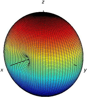
According to Eq. [SR], the overall radiation pattern of the antenna is the multiplication of the element pattern and the array pattern. The radiation pattern of a half-wave dipole antenna is calculated in the radiation section. For convenience it is also shown here in Fig. [2].
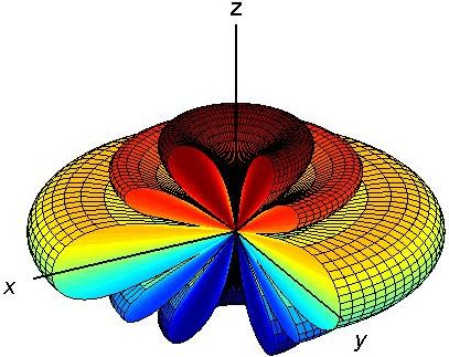
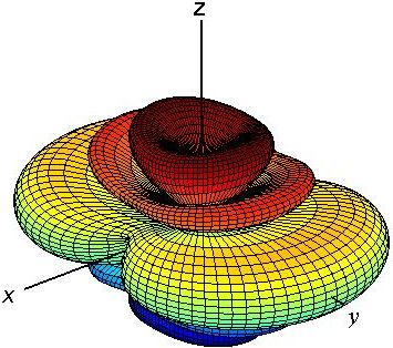
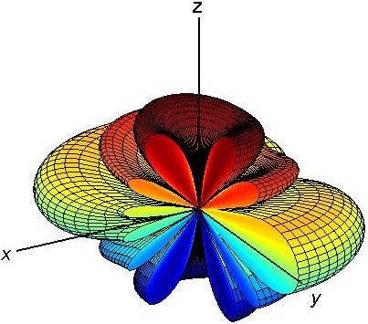
The array pattern is also shown in 3D in Fig. [3] (Note that the figures are plotted in dB in order to make the small side lobes visible). The overall pattern which is the multiplication of these two figures is shown in Fig. [4].
As can be seen the radiation pattern is much more directive than that of a single dipole antenna (compare Fig. [4] with [2]). In addition, it is no longer rotationally symmetric. Two cross sections of the overall pattern is shown in Fig. [5]. As can be seen the pattern has 6 lobes in x-z plane while it has 5 lobes y-z plane.