Tags: Permittivity / Legendre Polynomials / Boundary Conditions / Fröhlich Condition
![]() In this problem we will encounter the main physical features of dielectric spheres - their induced field and polarizability. The result is of great interest: understanding the interaction of light with small particles is one of the main concerns of nanophotonics. It leads to astonishing applications like cloaking, improvement of solar cells and lithography with extreme resolution.
In this problem we will encounter the main physical features of dielectric spheres - their induced field and polarizability. The result is of great interest: understanding the interaction of light with small particles is one of the main concerns of nanophotonics. It leads to astonishing applications like cloaking, improvement of solar cells and lithography with extreme resolution.
Problem Statement
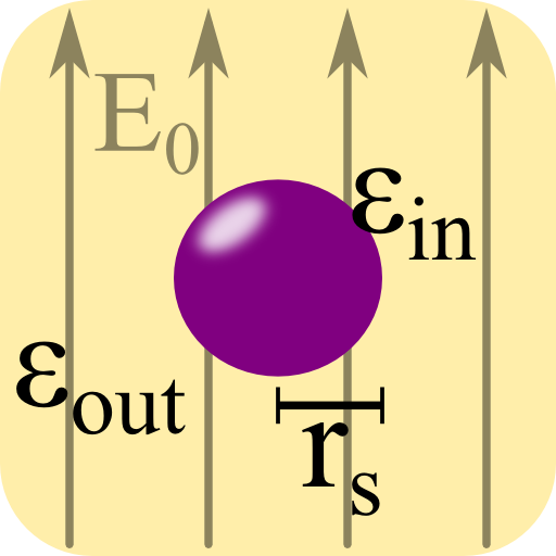
A dielectric sphere with radius rs and relative permittivity εin is embedded in a medium with relative permittivity εout.
The sphere is subject to a homogeneous electric field E(r) = E0ez.
Calculate the electrostatic potential in the entire space. Derive the polarizability α of the sphere from your result.
Hints
Which equation can be used to determine the electrostatic potential? What is a generel representation of the potential in spherical coordinates? Do you know a special set of functions that are already solutions to the governing equation?
How does the polarizability relate exciting and induced field?
A General Solution for the Potential
The strategy to find the solution for this problem is very general and used throughout the natural sciences. We will express the general solution of the guiding differential equation and solve the boundary conditions. Here, it is suitable to use the electrostatic potential \(\phi\), for which the Laplace equation holds if no charges are present:
\[\Delta\phi\left(\mathbf{r}\right) = 0\ .\]
Since the sphere is rotationally symmetric, it is convenient to treat the problem in spherical coordinates \(r\), \(\theta\) and \(\varphi\).
In spherical coordinates, the solution be can expressed in terms of Legendre polynomials \(P_{l}\left(\cos\theta\right)\).
The Laplace equation is fullfilled both by \(r^{l}P_{l}\left(\cos\theta\right)\) and \(P_{l}\left(\cos\theta\right)/r^{l+1}\) for all \(l=0\dots\infty\).
We have left out any dependency in \(\varphi\) since the exciting field is invariant in this angular direction. If this would not have been the case, we should have use spherical harmonics \(Y_{lm}\left(\theta,\varphi\right)\). The index m then denotes an angular variation of \(\exp\left(\mathrm{i}m\varphi\right)\). A constant function in φ, as in our case, is thus described by m = 0 and the \(Y_{l0}\) should be related to the \(P_{l}\) by a constant factor which is indeed the case.
The overall potential will be a superposition of the exciting potential and the potential of the sphere. Furthermore, inside the sphere, the field should be finite allowing only solutions in \(r^{l}\) whereas the same condition leads to the solutions with \(r^{-l-1}\) outside of it.
Hence we make the following ansatz for the potentials:
\[\begin{eqnarray*}\phi_{\mathrm{in}}\left(r,\theta\right) & = & \sum_{l=0}^{\infty}A_{l}r^{l}P_{l}\left(\cos\theta\right)\\ \phi_{\mathrm{out}}\left(r,\theta\right) & = & \underbrace{-E_{0}rP_{1}\left(\cos\theta\right)}_{\mathrm{exciting\ field}}\\ & & + \sum_{l=0}^{\infty}C_{l}P_{l} \left(\cos\theta\right)/r^{l+1}\ .\end{eqnarray*}\]
Employing the Boundary Conditions
The Al and Cl are constants we have to find employing the boundary conditions. Also, \(z=r\cos\theta\equiv rP_{1}\left(\cos\theta\right)\) and since \(\mathbf{E}_{\mathrm{exc}} \left(\mathbf{r}\right)=E_{0}\mathbf{e}_{z}=-\nabla\phi_{\mathrm{exc}}\left(\mathbf{r}\right)\) lead us to the given form of the exciting potential.
The regions in- and outside of the sphere have been denoted by the subscripts “in” and “out”, respectively, which will hold also for the rest of the solution.
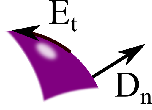 Now we have to use the boundary conditions. From \(\nabla\times\mathbf{E}\left(\mathbf{r}\right)=0\) we know that the tangential part of the electric field is continuous whereas \(\nabla\cdot \mathbf{D}\left(\mathbf{r}\right)=0\) implies that the normal part of \(\mathbf{D}\left(\mathbf{r}\right)\) is continuous, see also the figure on the right. Along with the constitutive relation \(\mathbf{D}\left(\mathbf{r}\right) = \varepsilon\left(\mathbf{r}\right)\mathbf{E}\left(\mathbf{r}\right)\) results in the continuity of \(\varepsilon\left( \mathbf{r}\right)\mathbf{E}\left( \mathbf{r}\right)\).
Using \(\mathbf{E}\left(\mathbf{r}\right) = -\nabla\phi\left(\mathbf{r}\right)\), we find
\[\begin{eqnarray*}-\frac{1}{r}\partial_{\theta}\phi_{\mathrm{in}} \left(r=r_{s},\theta\right) & = & -\frac{1}{r}\partial_{\theta}\phi_{\mathrm{out}}\left(r=r_{s},\theta\right) \\-\varepsilon_{\mathrm{i}}\partial_{r}\phi_{\mathrm{in}}\left(r=r_{s},\theta\right) & = & -\varepsilon_{\mathrm{o}}\partial_{r} \phi_{\mathrm{out}}\left(r=r_{s},\theta\right)\ .\end{eqnarray*}\]
Then, using
\[P_{l}^{1}\left(\cos\theta\right) = \frac{dP_{l}\left(\cos\theta\right)}{d\theta}\ ,\]
we get
\[\begin{eqnarray*}\partial_{\theta}\phi_{\mathrm{in}}\left(r=r_{s},\theta\right) & = & \sum_{l=1}^{\infty}A_{l}r_{s}^{l}P_{l}^{1} \left(\cos\theta\right)\\& \overset{!}{=} & -E_{0}r_{s}P_{1}^{1}\left(\cos\theta\right)\\& & +\sum_{l=1}^{\infty}C_{l}P_{l}^{1}\left(\cos\theta\right)/r_{s}^{l+1}\ .\end{eqnarray*}\]
The summation can start at \(l=1\) since \(P_{0}^{1}\left(x\right)=0\). Comparing the different series and using the orthogonality of the associated Legendre polynomials \(P_{l}^{m}\), we derive the relations
\[\begin{eqnarray*}A_{1}r_{s} & = & -E_{0}r_{s}+\frac{C_{1}}{r_{s}^{2}}\\A_{n}r_{s}^{2n+1} & = & C_{n}\ ,\ n\geq2\ .\end{eqnarray*}\]
Employing the second boundary condition

we can further conclude that
\[\begin{eqnarray*}0 & = & C_{0}\ ,\\ \varepsilon_{\mathrm{in}}\cdot A_{1} & = & -\varepsilon_{\mathrm{out}}\cdot\left(E_{0}+2C_{1}/r_{s}^{3}\right)\ \mathrm{and}\\ \varepsilon_{\mathrm{in}}nA_{n}r_{s}^{2n+1} & = & -\varepsilon_{\mathrm{out}}\left(n+1\right)C_{n}\ \mathrm{for}\ n\geq2\ .\end{eqnarray*}\]
This system of equations can only hold if \(A_{n}=C_{n}=0\) for all \(n\neq1\).
The remaining part can be formulated as
\[\left(\begin{array}{cc} r_{s}^{3} & -1\\ \frac{\varepsilon_{\mathrm{in}}}{\varepsilon_{\mathrm{out}}}r_{s}^{3} & 2 \end{array}\right)\left(\begin{array}{c} A_{1}\\ C_{1} \end{array}\right) = \left(\begin{array}{c} -E_{0}r_{s}^{3}\\ -E_{0}r_{s}^{3} \end{array}\right)\ .\]
This matrix-like representation seems a bit over the top for our task. This form, however, can be very useful if we want to generalize our approach to fields of arbitrary form. We can solve the latter equation to find
\[\begin{eqnarray*}A_{1} & = & -\frac{3E_{0}}{2+\varepsilon_{\mathrm{in}}/\varepsilon_{\mathrm{out}}}\\C_{1} & = & r_{s}^{3}E_{0}\frac{\varepsilon_{\mathrm{in}}- \varepsilon_{\mathrm{out}}} {\varepsilon_{\mathrm{in}}+2\varepsilon_{\mathrm{out}}}\ .\end{eqnarray*}\]
The Resulting Potential and Polarizability
We can put our findings now into the expression for the potential:
\[\begin{eqnarray*}\phi_{\mathrm{in}}\left(r,\theta\right) & = & -\frac{3E_{0}}{2+\varepsilon_{\mathrm{in}}/\varepsilon_{ \mathrm{out}}}\cdot rP_{1}\left(\cos\theta\right)\\ \phi_{\mathrm{out}}\left(r,\theta\right) & = & -E_{0}rP_{1}\left(\cos\theta\right)\\ & & +E_{0}\frac{\varepsilon_{\mathrm{in}}-\varepsilon_{\mathrm{out}}}{\varepsilon_{\mathrm{in}}+2\varepsilon_{\mathrm{out}}}\cdot\frac{r_{s}^{3}}{r^{2}}P_{1}\left(\cos\theta\right)\ . \end{eqnarray*}\]
Now, what is the polarizability \(\alpha\) of the sphere? Usually, this quantity is related to the dipole moment of an object subject to a constant electric field via \(\mathbf{p}=\alpha\mathbf{D}\). So, the only thing left to do is to relate our result do a dipole moment \(\mathbf{p}\) in the right units. The electrostatic potential of a dipole is given by
\[\phi_{\mathrm{dipole}}\left(\mathbf{r}\right) = \frac{1}{4\pi\varepsilon_{0}\varepsilon_{out}}\cdot\frac{\mathbf{p}\cdot\mathbf{r}}{r^{3}}\ .\]
We have to compare this dipole potential to the part of the sphere in \(\phi_{\mathrm{out}}\left(r,\theta\right)\). Since \(\mathbf{p}\cdot\mathbf{r}=prP_{1}\left(\cos\theta^{\prime}\right)\) with \(\theta^{\prime}\) being the angle between \(\mathbf{p}\) and \(\mathbf{r}\),
\[\begin{eqnarray*}\phi_{\mathrm{out}}^{\mathrm{sphere}}\left(r,\theta\right) & = & E_{0} \frac{\varepsilon_{\mathrm{in}}-\varepsilon_{\mathrm{out}}}{\varepsilon_{\mathrm{in}}+2\varepsilon_{ \mathrm{out}}}\cdot\frac{r_{s}^{3}}{r^{2}}P_{1}\left(\cos\theta\right)\\& \overset{!}{=} & \frac{1}{4\pi\varepsilon_{0} \varepsilon_{\mathrm{out}}}\cdot\frac{\mathbf{p} \cdot\mathbf{r}=prP_{1}\left(\cos\theta^{\prime}\right)}{r^{3}}\ .\end{eqnarray*}\]
So, we can conclude that \(\theta=\theta^{\prime}\) and also \(\mathbf{p}=p\mathbf{e}_{z}\) for our problem. In general, the polarizability of a sphere should not depend on the direction of the exciting field and we can write the result directly as
\[\begin{eqnarray*}\mathbf{p} & = & 4\pi r_{s}^{3}\cdot\varepsilon_{0}\varepsilon_{\mathrm{out}}\cdot\frac{\varepsilon_{\mathrm{in}}-\varepsilon_{\mathrm{out}}}{\varepsilon_{\mathrm{in}}+2\varepsilon_{\mathrm{out}}}\mathbf{E}_{0}\\ & \equiv & \varepsilon_{0}\varepsilon_{\mathrm{out}}\cdot\alpha\mathbf{E}_{0}\ \mathrm{with}\\ \alpha & = & 4\pi r_{s}^{3}\cdot\frac{\varepsilon_{\mathrm{in}}-\varepsilon_{\mathrm{out}}}{\varepsilon_{\mathrm{in}}+2\varepsilon_{\mathrm{out}}}\ . \end{eqnarray*} \]
The Fröhlich Condition and Cloaking Spheres
We have found a very important result that is at the heart of nanophotonics. If the denominator of \(\alpha\) vanishes, the system is said to have a dipole resonance. Then, the induced field of the sphere goes to infinity. For real media, however, one has to take into account also that the permittivity of the sphere can be a complex number implying losses and limiting the achievable induced field. Then, one defines the resonances by the minimum of \(\left|\varepsilon_{\mathrm{in}}+2\varepsilon_{\mathrm{out}}\right|\) which becomes for low \(\mathfrak{I}\left(\varepsilon_{\mathrm{in}}\right)\) approximately
\[\mathfrak{Re}\left(\varepsilon_{\mathrm{in}}+2\varepsilon_{\mathrm{out}}\right) = 0\ .\]
The latter equation is called the Fröhlich condition.
Using this result we can also explain the different polarization directions from the publication we discussed earlier in the background. If the sphere is a metal with \(-2\varepsilon_{\mathrm{out}}<\varepsilon_{\mathrm{in}}<-\varepsilon_{\mathrm{out}}\), the polarizability has a different sign than if it was a dielectric one with \(\varepsilon_{\mathrm{in}}>\varepsilon_{\mathrm{out}}\), for example for some glass in air. That means that the polarization fields of metallic and dielectric spheres, if arranged accordingly, may cancel each other - the dielectric sphere is cloaked as in “Cloaking dielectric spherical objects by a shell of metallic nanoparticles”. Naturally, losses in real metals and higher-order couplings will limit the effectivity of the cloak.
Background
The study of light-matter interactions is at the core of nanophotonics. Other than in classical optics, the investigated systems are only in the order of nanometers to a few microns. These systems are often made of basic building blocks like nanowires, rings with a gap (“split rings”), and spheres. Understanding these fundamental elements has lead to amazing new applications like the possibility to cloak certain regions from electromagnetic radiation.
For example, in “Cloaking dielectric spherical objects by a shell of metallic nanoparticles”, Physical Review B 83 (2011), the authors show how a dielectric sphere can be cloaked surrounding it by silver spheres. The principle behind the paper is that the polarization of a dielectric sphere and that of the silver spheres can have different signs. Then, finding the right parameters of the system, the induced fields cancel each other - the dielectric sphere is invisible!
Journal Page | arXiv | PDF


